Election Forecasting

In our model:

• The spread \(d∼N(\mu,\tau)\) describes our best guess in the absence of polling data. We set \(\mu=0\) (don't know who's going to win) and \(\tau=0.035\) (using historical data).

The average of observed data \(\bar{X}∣d∼N(d,\sigma)\) describes randomness due to sampling and the pollster effect.

Because the posterior distribution is normal, we can report a 95% credible interval that has a 95% chance of overlapping the parameter using E(p∣Y) and SE(p∣Y) .

Given an estimate of E(p∣Y) and SE(p∣Y) , we can use pnorm to compute the probability that d>0 .

It is common to see a general bias that affects all pollsters in the same way. This bias cannot be predicted or measured before the election. We will include a term in later models to account for this variability.

Code: Definition of results object

Code: Computing credible interval and probability

[1] 1

Mathematical Representations of Models

If we collect several polls with measured spreads \((X_1,...,X_j)\) with a sample size of N , these random variables have expected value \(d\) and standard error \(2\sqrt{p(1−p)/N}\).

For one polster we represent each measurement as \[X_j=d+\epsilon_j\] where

• j - index for diffferent polls
• d - actual spread of the election
• \(\epsilon\) - error assocaited with poll

Code: Simulated data for one pollster

Using data for several pollsters brings house effect (h) \[X_{ij}=d+h_i+\epsilon_{ij}\] where

• i - index for diffferent pollster
• h - house effect for each pollster

Code: Simulated data for several pollsters

In addition, there is a general bias affecting all pollsters (b) \[X_{ij}=d+b+h_i+\epsilon_{ij}\]

The sample average is now is \[\bar{X}=d+b+\frac{\sum_{i=1}^{N}X_i}{N}\]

Standard deviation is \[SE(\bar{X})=\sqrt{\sigma^2/N+\sigma_b^2}\]

The standard error of the general bias \(\sigma_b\) does not get reduced by averaging multiple polls, which increases the variability of our final estimate. If we redo the Bayesian calculation taking this variability into account, we get a result much closer to FiveThirtyEight’s:

Code: Computing credible interval and probability

[1] 0.817

Predicting the Electoral College

In the US election, each state has a certain number of votes that are won all-or-nothing based on the popular vote result in that state (with minor exceptions not discussed here).

We use the left_join() function to combine the number of electoral votes with our poll results. For each state, we apply a Bayesian approach to generate an Election Day d . We keep our prior simple by assuming an expected value of 0 and a standard deviation based on recent history of 0.02.

Code: Top 5 states ranked by electoral votes

1. > state electoral_votes clinton trump others
2. > 1 California 55 61.7 31.6 6.7
3. > 2 Texas 38 43.2 52.2 4.5
4. > 3 Florida 29 47.8 49.0 3.2
5. > 4 New York 29 59.0 36.5 4.5
6. > 5 Illinois 20 55.8 38.8 5.4
7. > 6 Pennsylvania 20 47.9 48.6 3.6

We use the left_join() function to combine the number of electoral votes with our poll results.

For each state, we apply a Bayesian approach to generate an Election Day d . We keep our prior simple by assuming an expected value of 0 and a standard deviation based on recent history of 0.02.

Code: Computing the average and standard deviation for each state

Code: Calculating the posterior mean and posterior standard error

We can run a Monte Carlo simulation that for each iteration simulates poll results in each state using that state's average and standard deviation, awards electoral votes for each state to Clinton if the spread is greater than 0, then compares the number of electoral votes won to the number of votes required to win the election (over 269).

Code: Monte Carlo simulation of Election Night results

[1] 0.998

If we include a general bias term, the estimated probability of Clinton winning decreases significantly.

Code: Monte Carlo simulation including general bias

[1] 0.848

Forecasting

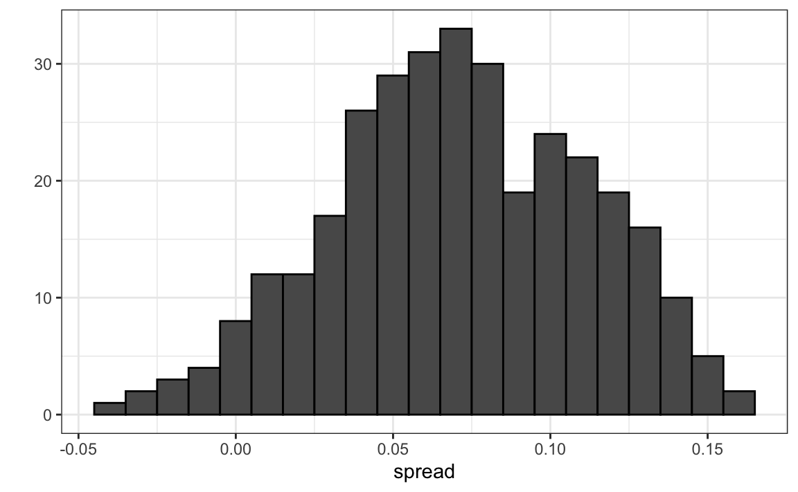
In poll results, p is not fixed over time. Variability within a single pollster comes from time variation.

Code: Variability across one pollster

1. > empirical theoretical
2. > 1 0.0403 0.0326

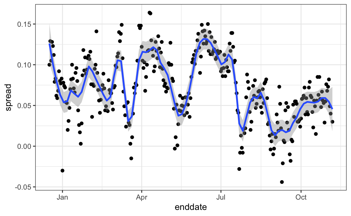
In order to forecast, our model must include a bias term \(b_t\) to model the time effect. Pollsters also try to estimate f(t) , the trend of p given time t using a model like: \[Y_{ij}=d+b+h_j+b_t+\epsilon_{ij}\]

Code: Trend across time for several pollsters

Once we decide on a model, we can use historical data and current data to estimate the necessary parameters to make predictions.

Election Forecasting - Exercises

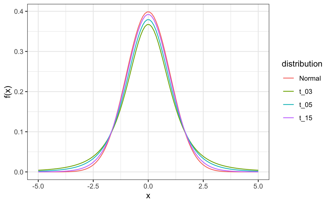
The t-Distribution

In models where we must estimate two parameters, p and σ, the Central Limit Theorem can result in overconfident confidence intervals for sample sizes smaller than approximately 30.

If the population data are known to follow a normal distribution, theory tells us how much larger to make confidence intervals to account for estimation of σ.

Given s as an estimate of σ , then \[Z=\frac{\bar{X}-d}{s\sqrt{N}} follows a t-distribution with N−1 degrees of freedom.

Degrees of freedom determine the weight of the tails of the distribution. Small values of degrees of freedom lead to increased probabilities of extreme values.

We can determine confidence intervals using the t-distribution instead of the normal distribution by calculating the desired quantile with the function qt().

Code: Calculating 95% confidence intervals with the t-distribution

[1] 2.14

[1] 1.96

The t-Distribution - Examples