We can use statistical theory to compute the probability that a given interval contains the true parameter p.
95% confidence intervals are intervals constructed to have a 95% chance of including p. The margin of error is approximately a 95% confidence interval.
The start and end of these confidence intervals are random variables. To calculate any size confidence interval, we need to calculate the value z for which \(Pr(−z≤Z≤z)\) equals the desired confidence. For example, a 99% confidence interval requires calculating z for \(Pr(−z≤Z≤z)=0.99\).
For a confidence interval of size q , we solve for \(z=1−\frac{1−q}{2}\) .
To determine a 95% confidence interval, use z <- qnorm(0.975). This value is slightly smaller than 2 times the standard error.
Code: Monte Carlo simulation of confidence intervals
N <- 1000
X <- sample(c(0,1), size = N, replace = TRUE, prob = c(1-p, p)) # generate N observations
X_hat <- mean(X) # calculate X_hat
SE_hat <- sqrt(X_hat*(1-X_hat)/N) # calculate SE_hat, SE of the mean of N observations
c(X_hat - 2*SE_hat, X_hat + 2*SE_hat) # build interval of 2*SE above and below mean
Code: geom_smooth confidence interval example
data.frame(year = as.numeric(time(nhtemp)), temperature = as.numeric(nhtemp)) %>%
ggplot(aes(year, temperature)) +
geom_point() +
geom_smooth() +
ggtitle("Average Yearly Temperatures in New Haven")
We can run a Monte Carlo simulation to confirm that a 95% confidence interval contains the true value of p 95% of the time.
Code: Monte Carlo simulation
inside <- replicate(B, {
X <- sample(c(0,1), size = N, replace = TRUE, prob = c(1-p, p))
X_hat <- mean(X)
SE_hat <- sqrt(X_hat*(1-X_hat)/N)
between(p, X_hat - 2*SE_hat, X_hat + 2*SE_hat) # TRUE if p in confidence interval
})
mean(inside)
A plot of confidence intervals from this simulation demonstrates that most intervals include p , but roughly 5% of intervals miss the true value of p.
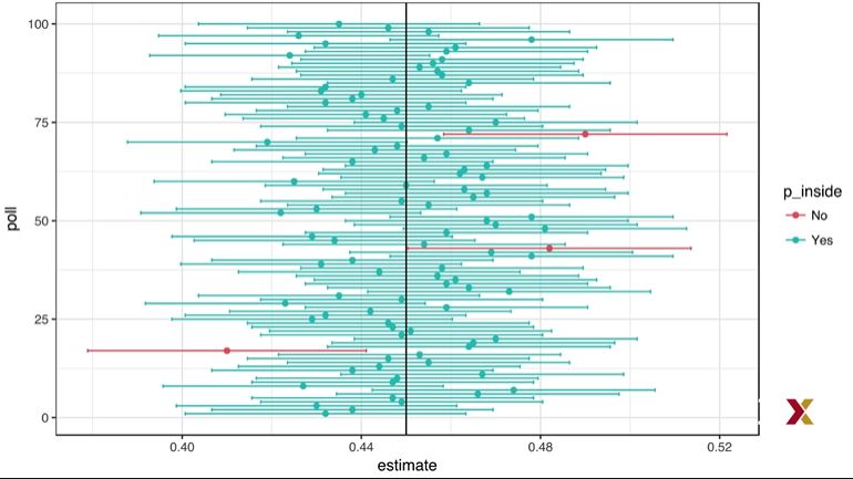
The 95% confidence intervals are random, but p is not random. 95% refers to the probability that the random interval falls on top of p . It is technically incorrect to state that p has a 95% chance of being in between two values because that implies p is random.
Power
If we are trying to predict the result of an election, then a confidence interval that includes a spread of 0 (a tie) is not helpful. A confidence interval that includes a spread of 0 does not imply a close election, it means the sample size is too small.
Power is the probability of detecting an effect when there is a true effect to find. Power increases as sample size increases, because larger sample size means smaller standard error.
Code: Confidence interval for the spread with sample size of 25
X_hat <- 0.48
(2*X_hat - 1) + c(-2, 2)*2*sqrt(X_hat*(1-X_hat)/N)
p-Values
The null hypothesis is the hypothesis that there is no effect. In this case, the null hypothesis is that the spread is 0, or p=0.5 .
The p-value is the probability of detecting an effect of a certain size or larger when the null hypothesis is true. We can convert the probability of seeing an observed value under the null hypothesis into a standard normal random variable. We compute the value of z that corresponds to the observed result, and then use that z to compute the p-value.
If a 95% confidence interval does not include our observed value, then the p-value must be smaller than 0.05. It is preferable to report confidence intervals instead of p-values, as confidence intervals give information about the size of the estimate and p-values do not.
Code: p-value for observed spread of 0.02
z <- sqrt(N) * 0.02/0.5 # spread of 0.02
1 - (pnorm(z) - pnorm(-z))
The p-value is the probability of observing a value as extreme or more extreme than the result given that the null hypothesis is true.
In the context of the normal distribution, this refers to the probability of observing a Z-score whose absolute value is as high or higher than the Z-score of interest.
Suppose we want to find the p-value of an observation 2 standard deviations larger than the mean. This means we are looking for anything with \(∣z∣≥2\) .
Graphically, the p-value gives the probability of an observation that's at least as far away from the mean or further. This plot shows a standard normal distribution (centered at z=0 with a standard deviation of 1). The shaded tails are the region of the graph that are 2 standard deviations or more away from the mean.
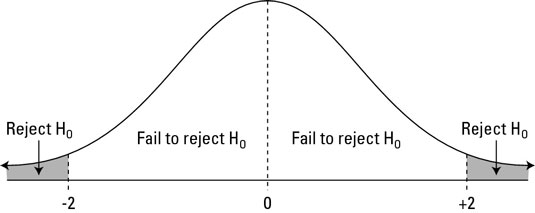
The right tail can be found with \(1-pnorm(2)\). We want to have both tails, though, because we want to find the probability of any observation as far away from the mean or farther, in either direction. (This is what's meant by a two-tailed p-value.) Because the distribution is symmetrical, the right and left tails are the same size and we know that our desired value is just \(2\dot(1-pnorm(2))\).