Prerequisites
library(dplyr)
library(ggplot2)
1. Confidence interval for p
We will use all the national polls that ended within a few weeks before the election.
Assume there are only two candidates and construct a 95% confidence interval for the election night proportion.
- Use filter to subset the data set for the poll data you want. Include polls that ended on or after October 31, 2016 (enddate). Only include polls that took place in the United States. Call this filtered object polls.
- Use nrow to make sure you created a filtered object polls that contains the correct number of rows.
- Extract the sample size N from the first poll in your subset object polls.
- Convert the percentage of Clinton voters (rawpoll_clinton) from the first poll in polls to a proportion, X_hat. Print this value to the console.
- Find the standard error of X_hat given N. Print this result to the console.
- Calculate the 95% confidence interval of this estimate using the qnorm function.
- Save the lower and upper confidence intervals as an object called ci. Save the lower confidence interval first.
data(polls_us_election_2016)
# Generate an object `polls` that contains data filtered for polls that ended on or after October 31, 2016 in the United States
polls <- filter(polls_us_election_2016, enddate>='2016-10-31' & state =='U.S.')
# How many rows does `polls` contain? Print this value to the console.
nrow(polls)
[1] 70
N <- polls$samplesize[1]
N
[1] 2220
X_hat <- polls$rawpoll_clinton[1] /100
X_hat
[1] 0.47
se_hat <-sqrt(X_hat*(1-X_hat)/N)
se_hat
[1] 0.01059279
f <- qnorm(0.975)
ci <- c(X_hat-f*se_hat, X_hat+f*se_hat)
2. Pollster results for p
Create a new object called pollster_results that contains the pollster's name, the end date of the poll, the proportion of voters who declared a vote for Clinton, the standard error of this estimate, and the lower and upper bounds of the confidence interval for the estimate.
- Use the mutate function to define four new columns: X_hat, se_hat, lower, and upper. Temporarily add these columns to the polls object that has already been loaded for you.
- In the X_hat column, convert the raw poll results for Clinton to a proportion.
- In the se_hat column, calculate the standard error of X_hat for each poll using the sqrt function.
- In the lower column, calculate the lower bound of the 95% confidence interval using the qnorm function.
- In the upper column, calculate the upper bound of the 95% confidence interval using the qnorm function.
- Use the select function to select the columns from polls to save to the new object pollster_results.
head(polls)
# Create a new object called `pollster_results` that contains columns for pollster name, end date, X_hat, se_hat, lower confidence interval, and upper confidence interval for each poll.
polls <- mutate(polls, X_hat = polls$rawpoll_clinton /100, se_hat =sqrt(X_hat*(1-X_hat)/samplesize), lower=X_hat-qnorm(0.975)*se_hat, upper=X_hat+qnorm(0.975)*se_hat)
pollster_results <- select(polls, pollster, enddate, X_hat, se_hat, lower, upper)
3. Comparing to actual results - p
The final tally for the popular vote was Clinton 48.2% and Trump 46.1%. Add a column called hit to pollster_results that states if the confidence interval included the true proportion or not. What proportion of confidence intervals included?
- Finish the code to create a new object called avg_hit by following these steps.
- Use the mutate function to define a new variable called 'hit'.
- Use logical expressions to determine if each values in lower and upper span the actual proportion.
- Use the mean function to determine the average value in hit and summarize the results using summarize.
head(pollster_results)
# Add a logical variable called `hit` that indicates whether the actual value exists within the confidence interval of each poll. Summarize the average `hit` result to determine the proportion of polls with confidence intervals include the actual value. Save the result as an object called `avg_hit`.
avg_hit <- mutate(pollster_results, hit = (lower < 0.482 & upper > 0.482)) %>% summarize(mean(hit))
avg_hit
mean(hit)
1 0.3142857
4. Confidence interval for d
A much smaller proportion of the polls than expected produce confidence intervals containing p. Notice that most polls that fail to include p are underestimating. The rationale for this is that undecided voters historically divide evenly between the two main candidates on election day.
In this case, it is more informative to estimate the spread or the difference between the proportion of two candidates d, or \(0.482-0.461=0.021\) for this election.
Assume that there are only two parties and that \(d=2p-1\). Construct a 95% confidence interval for difference in proportions on election night.
- Use the mutate function to define a new variable called 'd_hat' in polls as the proportion of Clinton voters minus the proportion of Trump voters.
- Extract the sample size N from the first poll in your subset object polls.
- Extract the difference in proportions of voters d_hat from the first poll in your subset object polls.
- Use the formula above to calculate from d_hat. Assign to the variable X_hat.
- Find the standard error of the spread given N. Save this as se_hat.
- Calculate the 95% confidence interval of this estimate of the difference in proportions, d_hat, using the qnorm function.
- Save the lower and upper confidence intervals as an object called ci. Save the lower confidence interval first.
polls <- polls_us_election_2016 %>% filter(enddate >= "2016-10-31" & state == "U.S.") %>% mutate(d_hat = rawpoll_clinton/100 - rawpoll_trump/100)
# Assign the sample size of the first poll in `polls` to a variable called `N`. Print this value to the console.
N <- polls$samplesize[1]
N
[1] 2220
d_hat <- polls$d_hat[1]
d_hat
[1] 0.04
X_hat <- (d_hat+1)/2
# Calculate the standard error of the spread and save it to a variable called `se_hat`. Print this value to the console.
se_hat <- 2*sqrt(X_hat*(1-X_hat)/N)
# Use `qnorm` to calculate the 95% confidence interval for the difference in the proportions of voters. Save the lower and then the upper confidence interval to a variable called `ci`.
ci <- c(d_hat - qnorm(0.975)*se_hat, d_hat + qnorm(0.975)*se_hat)
5. Pollster results for d
Create a new object called pollster_results that contains the pollster's name, the end date of the poll, the difference in the proportion of voters who declared a vote either, and the lower and upper bounds of the confidence interval for the estimate.
- Use the mutate function to define four new columns: 'X_hat', 'se_hat', 'lower', and 'upper'. Temporarily add these columns to the polls object that has already been loaded for you.
- In the X_hat column, calculate the proportion of voters for Clinton using d_hat.
- In the se_hat column, calculate the standard error of the spread for each poll using the sqrt function.
- In the lower column, calculate the lower bound of the 95% confidence interval using the qnorm function.
- In the upper column, calculate the upper bound of the 95% confidence interval using the qnorm function.
- Use the select function to select the pollster, enddate, d_hat, lower, upper columns from polls to save to the new object pollster_results.
head(polls)
# Create a new object called `pollster_results` that contains columns for pollster name, end date, d_hat, lower confidence interval of d_hat, and upper confidence interval of d_hat for each poll.
pollster_results <- polls %>% mutate(X_hat = (d_hat + 1) / 2) %>% mutate(se_hat = 2 * sqrt(X_hat * (1 - X_hat) / samplesize)) %>% mutate(lower = d_hat - qnorm(0.975) * se_hat) %>% mutate(upper = d_hat + qnorm(0.975) * se_hat) %>% select(pollster, enddate, d_hat, lower, upper)
6. Comparing to actual results - d
What proportion of confidence intervals for the difference between the proportion of voters included d, the actual difference in election day?
- Use the mutate function to define a new variable within pollster_results called hit.
- Use logical expressions to determine if each values in lower and upper span the actual difference in proportions of voters.
- Use the mean function to determine the average value in hit and summarize the results using summarize.
- Save the result of your entire line of code as an object called avg_hit.
head(pollster_results)
# Add a logical variable called `hit` that indicates whether the actual value (0.021) exists within the confidence interval of each poll. Summarize the average `hit` result to determine the proportion of polls with confidence intervals include the actual value. Save the result as an object called `avg_hit`.
avg_hit <- mutate(pollster_results, hit = (lower < 0.021 & upper > 0.021)) %>% summarize(mean(hit))
avg_hit
mean(hit)
1 0.7714286
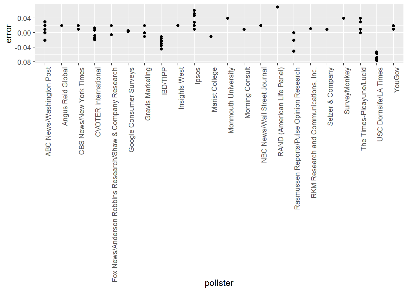
7. Comparing to actual results by pollster
Although the proportion of confidence intervals that include the actual difference between the proportion of voters increases substantially, it is still lower that 0.95. In the next chapter, we learn the reason for this.
To motivate our next exercises, calculate the difference between each poll's estimate \(\bar{d}\)
and the actual \(d=0.021\). Stratify this difference, or error, by pollster in a plot.
- Define a new variable errors that contains the difference between the estimated difference between the proportion of voters and the actual difference on election day, 0.021.
- To create the plot of errors by pollster, add a layer with the function geom_point. The aesthetic mappings require a definition of the x-axis and y-axis variables. So the code looks like the example below, but you fill in the variables for x and y.
- The last line of the example code adjusts the x-axis labels so that they are easier to read.
head(polls)
# Add variable called `error` to the object `polls` that contains the difference between d_hat and the actual difference on election day. Then make a plot of the error stratified by pollster.
polls <- mutate(polls, error=(d_hat-0.021) )
polls %>% ggplot(aes(x = pollster, y = error)) + geom_point() + theme(axis.text.x = element_text(angle = 90, hjust = 1))
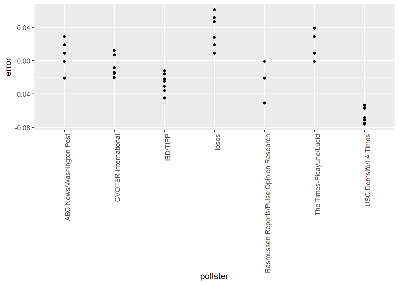
8. Comparing to actual results by pollster - multiple polls
Remake the plot you made for the previous exercise, but only for pollsters that took five or more polls.
You can use dplyr tools group_by and n to group data by a variable of interest and then count the number of observations in the groups. The function filter filters data piped into it by your specified condition.
- Define a new variable errors that contains the difference between the estimated difference between the proportion of voters and the actual difference on election day, 0.021.
- Group the data by pollster using the group_by function.
- Filter the data by pollsters with 5 or more polls.
- Use ggplot to create the plot of errors by pollster.
- Add a layer with the function geom_point.
head(polls)
# Add variable called `error` to the object `polls` that contains the difference between d_hat and the actual difference on election day. Then make a plot of the error stratified by pollster, but only for pollsters who took 5 or more polls.
polls %>% mutate(error = d_hat - 0.021) %>%
group_by(pollster) %>%
filter(n() >= 5) %>%
ggplot(aes(pollster, error)) +
geom_point() +
theme(axis.text.x = element_text(angle = 90, hjust = 1))