Because \(\bar{X}\) is the sum of random draws divided by a constant, the distribution of \(\bar{X}\) is approximately normal.
We can convert \(\bar{X}\) to a standard normal random variable Z : \[Z=\frac{\bar{X}-E(\bar{X})}{SE(\bar{X})}\]
The probability that \(\bar{X}\) is within .01 of the actual value of p is: \[Pr(Z\leq0.01/\sqrt{p(1-p)/N)}-Pr(Z\leq-0.01/\sqrt{p(1-p)/N)}\]
The Central Limit Theorem (CLT) still works if \(\bar{X}\) is used in place of p . This is called a plug-in estimate. Hats over values denote estimates. Therefore:
\[\hat{SE}(\bar{X})=\sqrt{\bar{X}(1-\bar{X})/N}\]
Using the CLT, the probability that \(\bar{X}\) is within .01 of the actual value of p is:
\[Pr(Z\leq0.01/\sqrt{\bar{X}(1-\bar{X})/N)}-Pr(Z\leq-0.01/\sqrt{\bar{X}(1-\bar{X})/N)}\]
Computing the probability of \(\bar{X}\) being within .01 of p
se <- sqrt(X_hat*(1-X_hat)/25)
pnorm(0.01/se) - pnorm(-0.01/se)
Margin of Error
The margin of error is defined as 2 times the standard error of the estimate \(\bar{X}\) . There is about a 95% chance that \(\bar{X}\) will be within two standard errors of the actual parameter p
A Monte Carlo Simulation for the CLT
We can run Monte Carlo simulations to compare with theoretical results assuming a value of p . In practice, p is unknown. We can corroborate theoretical results by running Monte Carlo simulations with one or several values of p .
One practical choice for p when modeling is \(\bar{X}\) , the observed value of \(\hat{X}\) in a sample.
Code: Monte Carlo simulation using a set value of p
N <- 1000
# simulate one poll of size N and determine x_hat
x <- sample(c(0,1), size = N, replace = TRUE, prob = c(1-p, p))
x_hat <- mean(x)
# simulate B polls of size N and determine average x_hat
B <- 10000 # number of replicates
N <- 1000 # sample size per replicate
x_hat <- replicate(B, {
x <- sample(c(0,1), size = N, replace = TRUE, prob = c(1-p, p))
mean(x)
})
Code: Histogram and QQ-plot of Monte Carlo results
library(gridExtra)
p1 <- data.frame(x_hat = x_hat) %>%
ggplot(aes(x_hat)) +
geom_histogram(binwidth = 0.005, color = "black")
p2 <- data.frame(x_hat = x_hat) %>%
ggplot(aes(sample = x_hat)) +
stat_qq(dparams = list(mean = mean(x_hat), sd = sd(x_hat))) +
geom_abline() +
ylab("X_hat") +
xlab("Theoretical normal")
grid.arrange(p1, p2, nrow=1)
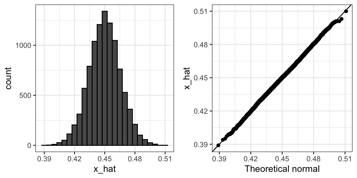
A histogram and qq-plot confirm that the normal approximation is accurate as well
The Spread
The spread between two outcomes with probabilities p and 1−p is 2p−1 .
The expected value of the spread is \(2\bar{X}−1\) .
The standard error of the spread is \(2\hat{SE}(\hat{X})\) .
The margin of error of the spread is 2 times the margin of error of \(\bar{X}\) .
Bias: Why Not Run a Very Large Poll?
An extremely large poll would theoretically be able to predict election results almost perfectly.These sample sizes are not practical. In addition to cost concerns, polling doesn't reach everyone in the population (eventual voters) with equal probability, and it also may include data from outside our population (people who will not end up voting). These systematic errors in polling are called bias.
Code: Plotting margin of error in an extremely large poll over a range of values of p
N <- 100000
p <- seq(0.35, 0.65, length = 100)
SE <- sapply(p, function(x) 2*sqrt(x*(1-x)/N))
data.frame(p = p, SE = SE) %>%
ggplot(aes(p, SE)) +
geom_line()