Poll aggregators combine the results of many polls to simulate polls with a large sample size and therefore generate more precise estimates than individual polls. Polls can be simulated with a Monte Carlo simulation and used to construct an estimate of the spread and confidence intervals.
Code: Simulating polls
Ns <- c(1298, 533, 1342, 897, 774, 254, 812, 324, 1291, 1056, 2172, 516)
p <- (d+1)/2
# calculate confidence intervals of the spread
confidence_intervals <- sapply(Ns, function(N){
X <- sample(c(0,1), size=N, replace=TRUE, prob = c(1-p, p))
X_hat <- mean(X)
SE_hat <- sqrt(X_hat*(1-X_hat)/N)
2*c(X_hat, X_hat - 2*SE_hat, X_hat + 2*SE_hat) - 1
})
# generate a data frame storing results
polls <- data.frame(poll = 1:ncol(confidence_intervals),
t(confidence_intervals), sample_size = Ns)
names(polls) <- c("poll", "estimate", "low", "high", "sample_size")
polls
Code: Calculating the spread of combined polls
summarize(avg = sum(estimate*sample_size) / sum(sample_size)) %>%.$avg #$
p_hat <- (1+d_hat)/2
moe <- 2*1.96*sqrt(p_hat*(1-p_hat)/sum(polls$sample_size))
round(d_hat*100,1)
round(moe*100, 1)
The actual data science exercise of forecasting elections involves more complex statistical modeling, but these underlying ideas still apply.
Pollsters and Multilevel Models
Different poll aggregators generate different models of election results from the same poll data. This is because they use different statistical models.
We will use actual polling data about the popular vote from the 2016 US presidential election to learn the principles of statistical modeling.
Poll Data and Pollster Bias
We analyze real 2016 US polling data organized by FiveThirtyEight. We start by using reliable national polls taken within the week before the election to generate an urn model.
Consider p the proportion voting for Clinton and 1−p the proportion voting for Trump. We are interested in the spread \(d=2p−1\).
Poll results are a random normal variable with expected value of the spread d and standard error \(2p\sqrt{(1−p)/N}\).
Code: Generating simulated poll data
data(polls_us_election_2016)
names(polls_us_election_2016)
# keep only national polls from week before election with a grade considered reliable
polls <- polls_us_election_2016 %>%
filter(state == "U.S." & enddate >= "2016-10-31" &
(grade %in% c("A+", "A", "A-", "B+") | is.na(grade)))
# add spread estimate
polls <- polls %>%
mutate(spread = rawpoll_clinton/100 - rawpoll_trump/100)
# compute estimated spread for combined polls
d_hat <- polls %>%
summarize(d_hat = sum(spread * samplesize) / sum(samplesize)) %>%
.$d_hat #$
# compute margin of error
p_hat <- (d_hat+1)/2
moe <- 1.96 * 2 * sqrt(p_hat*(1-p_hat)/sum(polls$samplesize))
# histogram of the spread
polls %>%
ggplot(aes(spread)) +
geom_histogram(color="black", binwidth = .01)
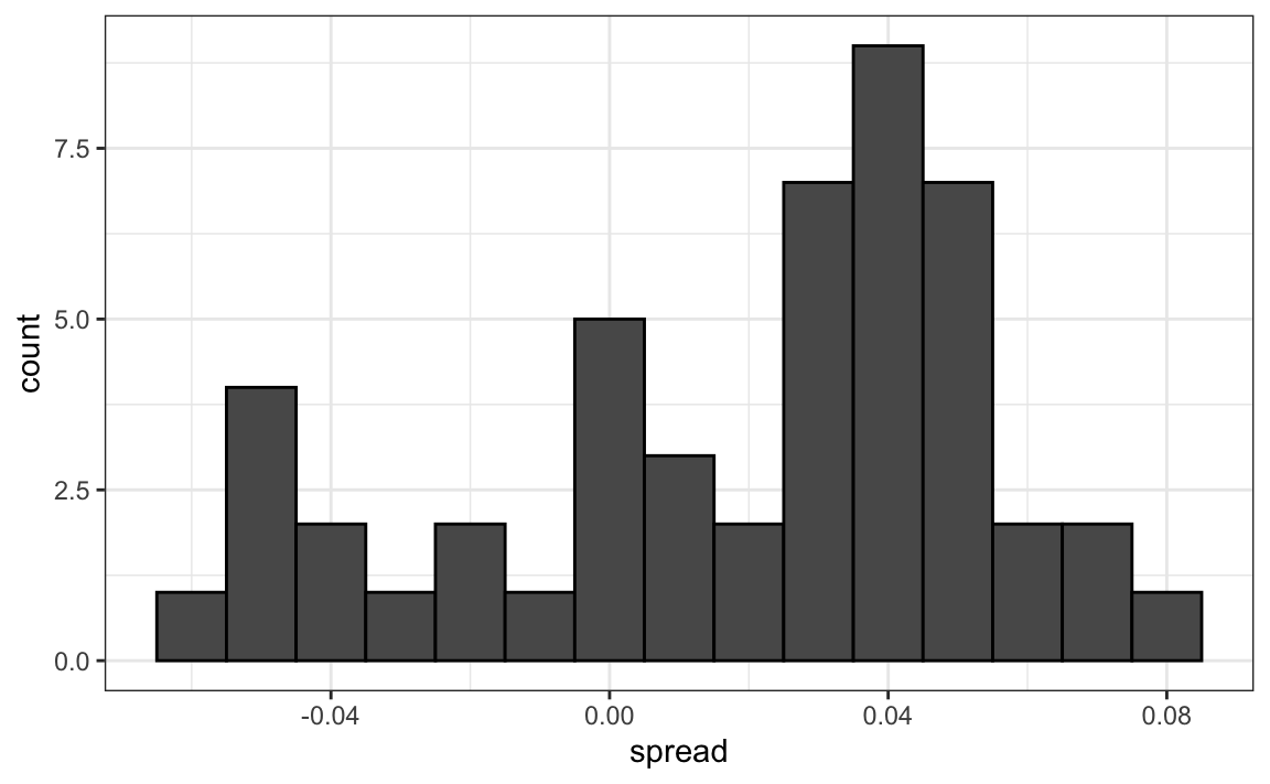
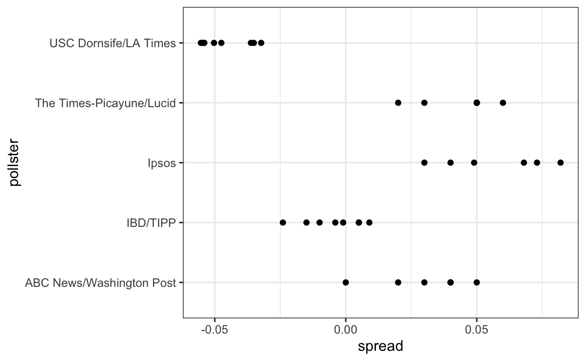
Our initial estimate of the spread did not include the actual spread. Part of the reason is that different pollsters have different numbers of polls in our dataset, and each pollster has a bias. Pollster bias reflects the fact that repeated polls by a given pollster have an expected value different from the actual spread and different from other pollsters. Each pollster has a different bias.
Code: Investigating poll data and pollster bias
polls %>% group_by(pollster) %>% summarize(n())
# plot results by pollsters with at least 6 polls
polls %>% group_by(pollster) %>%
filter(n() >= 6) %>%
ggplot(aes(pollster, spread)) +
geom_point() +
theme(axis.text.x = element_text(angle = 90, hjust = 1))
# standard errors within each pollster
polls %>% group_by(pollster) %>%
filter(n() >= 6) %>%
summarize(se = 2 * sqrt(p_hat * (1-p_hat) / median(samplesize)))
The urn model does not account for pollster bias. We will develop a more flexible data-driven model that can account for effects like bias.
Data-Driven Models
Instead of using an urn model where each poll is a random draw from the same distribution of voters, we instead define a model using an urn that contains poll results from all possible pollsters.
We assume the expected value of this model is the actual spread \(d=2p−1\) . Our new standard error σ now factors in pollster-to-pollster variability. It can no longer be calculated from p or d and is an unknown parameter.
The central limit theorem still works to estimate the sample average of many polls X1,...,XN because the average of the sum of many random variables is a normally distributed random variable with expected value d and standard error \(\sigma/\sqrt{N}\).
We can estimate the unobserved σ as the sample standard deviation, which is calculated with the sd function. \[\sigma=\frac{\sum_{i=1}^{N}\left (X_i-\bar{X} \right )}{\left( N-1 \right )} \]
Code
one_poll_per_pollster <- polls %>% group_by(pollster) %>%
filter(enddate == max(enddate)) %>% # keep latest poll
ungroup()
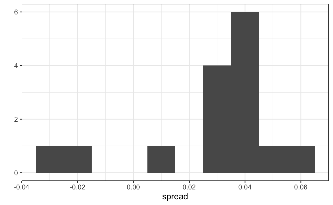
# histogram of spread estimates
one_poll_per_pollster %>%
ggplot(aes(spread)) + geom_histogram(binwidth = 0.01)
# construct 95% confidence interval
results <- one_poll_per_pollster %>%
summarize(avg = mean(spread), se = sd(spread)/sqrt(length(spread))) %>%
mutate(start = avg - 1.96*se, end = avg + 1.96*se)
round(results*100, 1)